Diagram layout engines: Minimizing hierarchical edge crossings

TALA is a new layout engine designed specifically for software architecture. At its core, it combines many different graph visualization algorithms to produce aesthetic diagrams. This article is a part of a series where we dive into the inner workings of TALA.

Today's topic is on minimizing edge crossings in hierarchical layouts.

For background, a hierarchical layout is a diagram that splits all the objects into layers of a hierarchy in one direction, e.g. top-down being the most typical. Many layout engines such as Graphviz's DOT are only hierarchical, meaning your diagram will be a hierarchy whether or not the model you intended is hierarchical in nature. TALA, on the other hand, identifies portions of the diagram which appear to be hierarchical, and selectively applies a hierarchical layout algorithm to those portions.

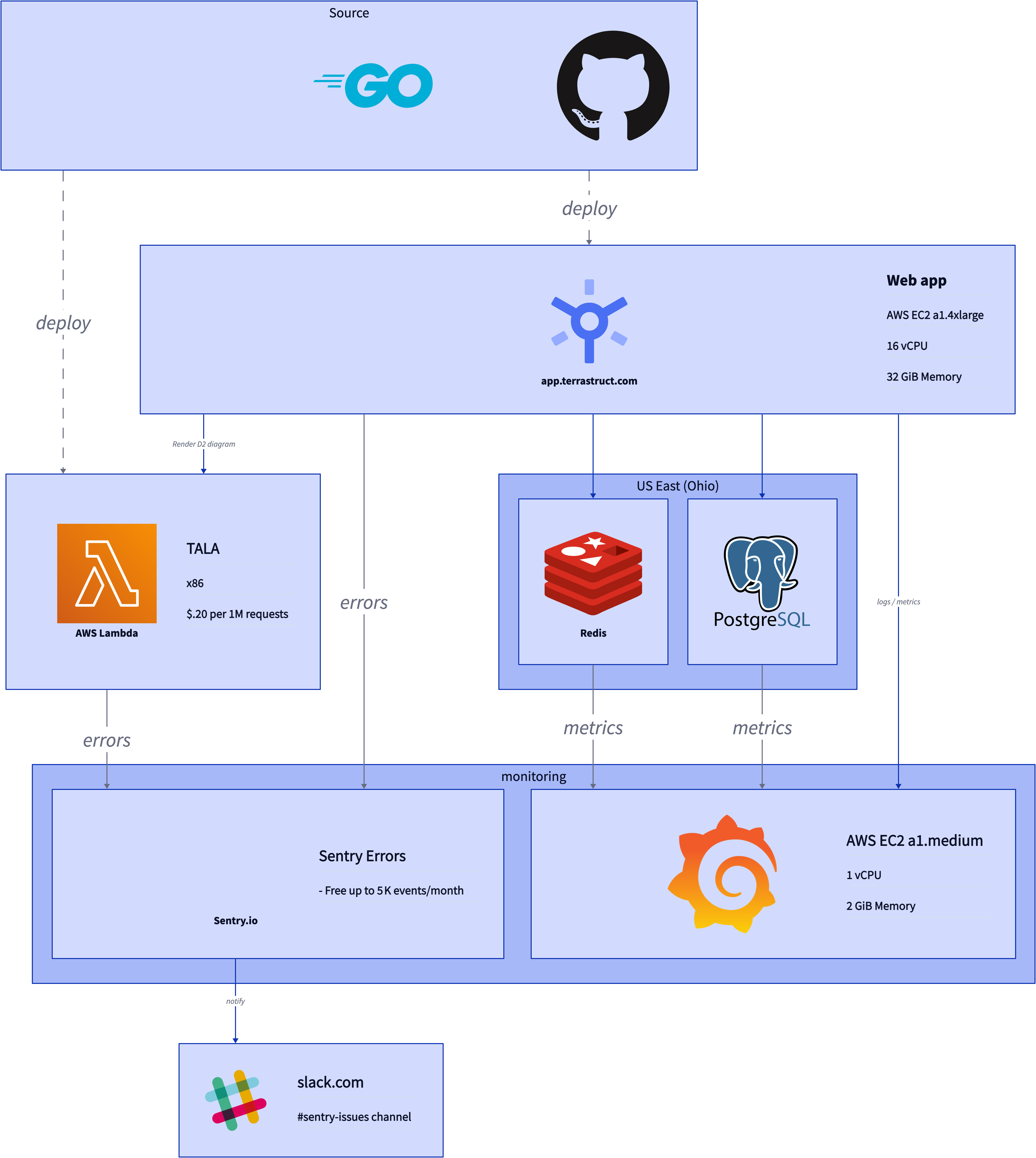
An example hierarchical diagram rendered by TALA.

The Problem

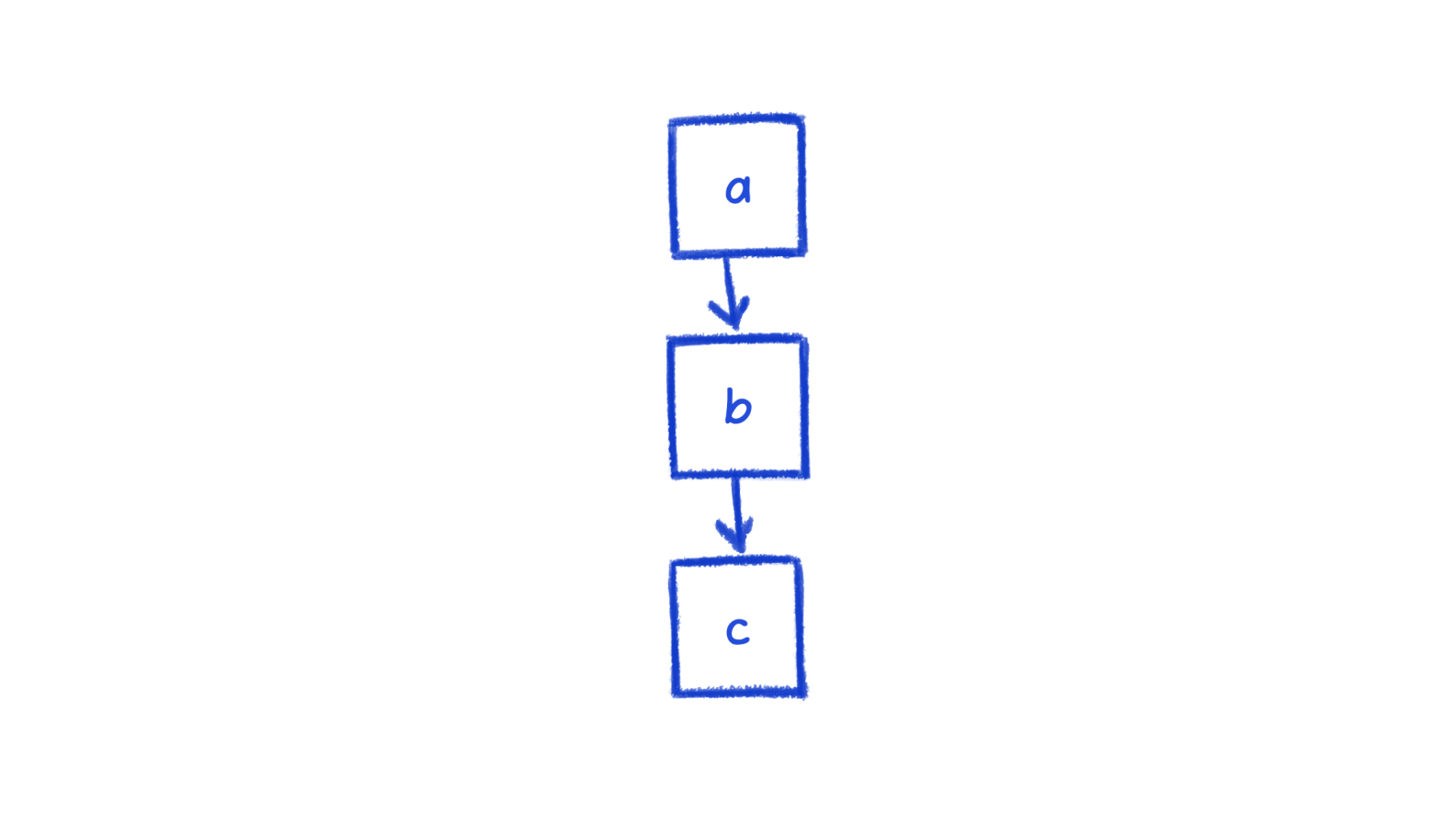
Let's start with the most basic hierarchy: a -> b -> c. There's only one way to arrange this hierarchically (assuming top-down).

Now let's throw in 2 more objects.

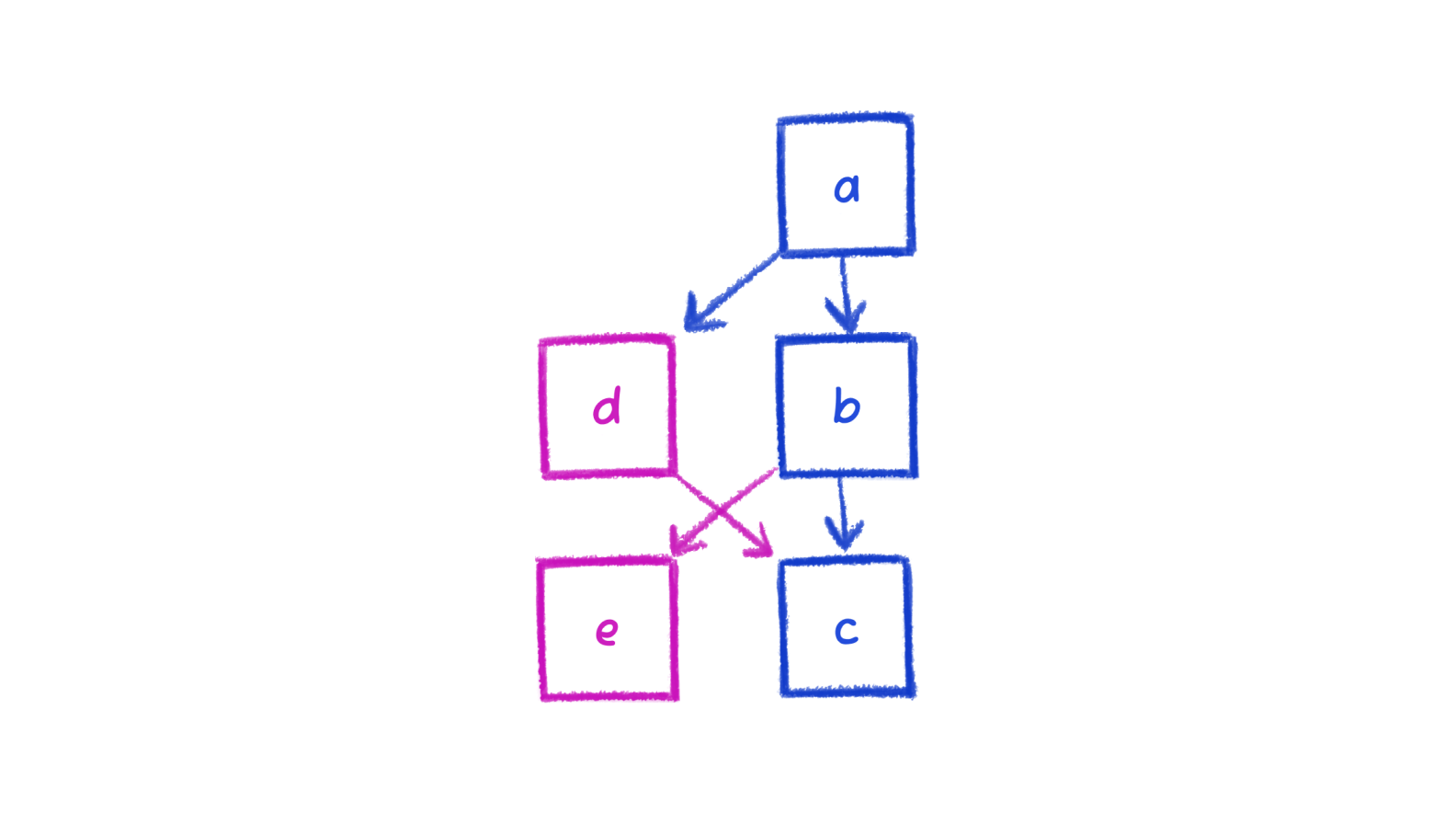
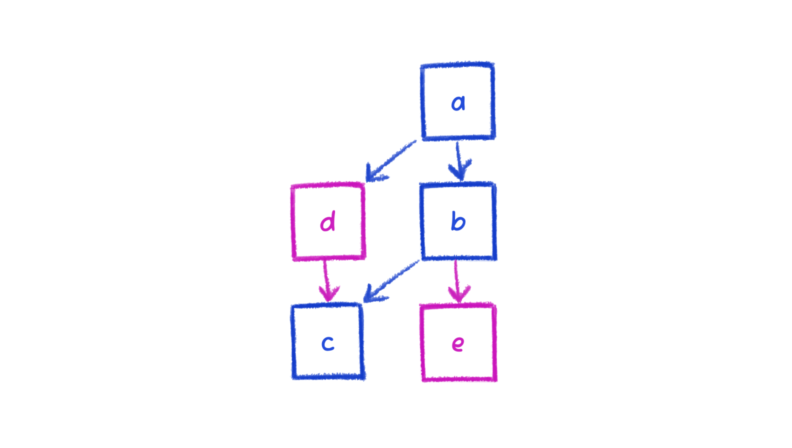
There is now more than just the one way to arrange. You can swap the nodes in the second or third layers, move a to the left, move nodes to other layers.

All else being equal, the layout engine should choose the arrangement that minimizes edge crossings. In general, fewer edge crossings means a cleaner and preferred layout.

We can quite easily see that a swap in either the second or third layer results in fewer crossings.

What about this diagram? Can you see what needs to rearrange to optimize this?

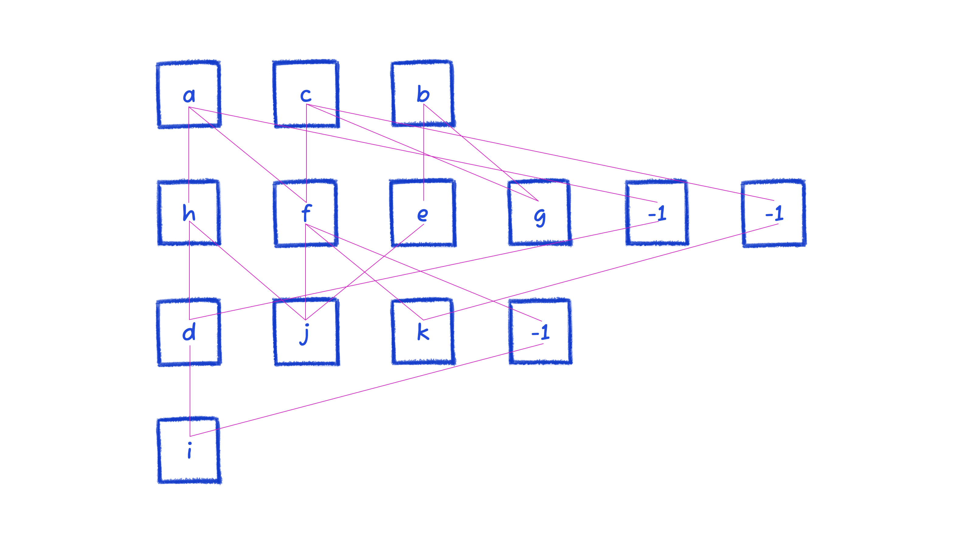
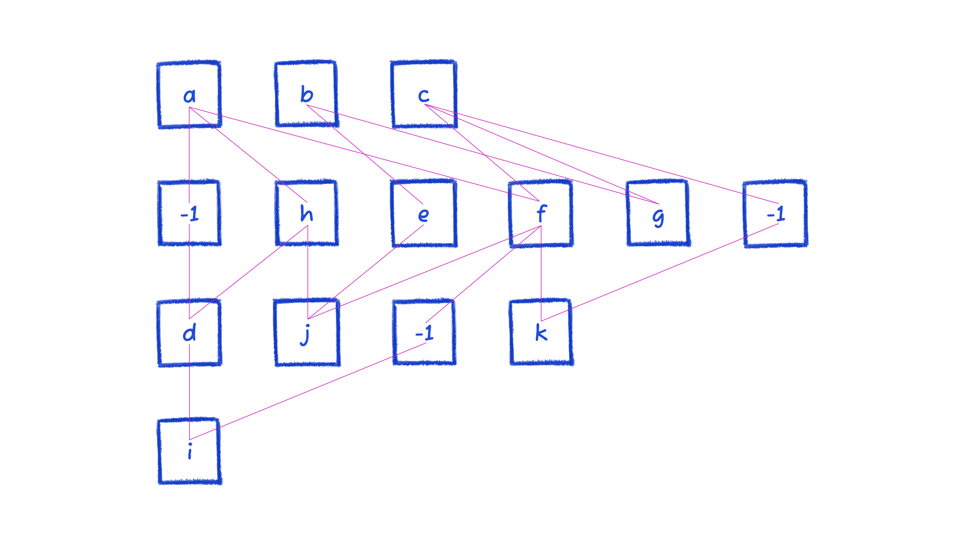
When the diagram gets larger, it's not easy to find the swaps and movements to reduce crossings. We certainly can't eyeball it. This type of problem is NP-hard: there’s no algorithm that’ll give an optimal solution for all cases in a reasonable runtime. So we approximate with heuristics. The crossing minimization steps covered in this article rearrange the above diagram such that the number of crossings is reduced from the 12 (pictured above), to the 2 (pictured below).

Assumptions

By the time the diagram reaches the crossing-minimization stage of this article, it has already passed through some relevant stages:

1. Hierarchy identification
2. Connection-breaking
3. Layer assignment

These are meaty enough to be posts of their own, so we'll keep the explanations of them brief. Also note that there are stages that run after this, so what we arrive at isn't the end result of the entire engine.

Hierarchy identification

This stage asks questions to identify whether a subgraph should use the hierarchical layout algorithms. For example, does this subgraph have majority connections flowing in one direction? If not, a hierarchy is likely a poor choice of layout. Does it contain special shapes? If it has a sequence of steps, that takes precedence over hierarchies.

Connection-breaking

Dummy nodes are nodes inserted in between long connections. They exist only for the span of crossing minimization.

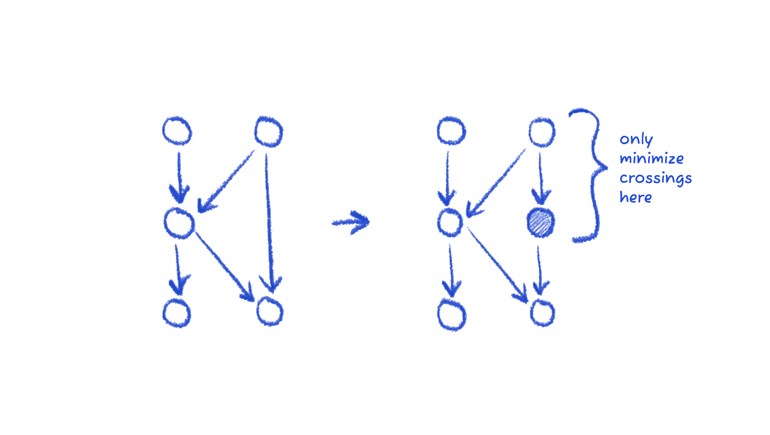
This helps cross-minimization localize its algorithm layer-by-layer, instead of having to consider adjacent nodes that skip layers.

Dummy nodes are represented with -1 throughout this article.

Layer assignment

This stage turns a list of connected nodes and assigns them their layers.

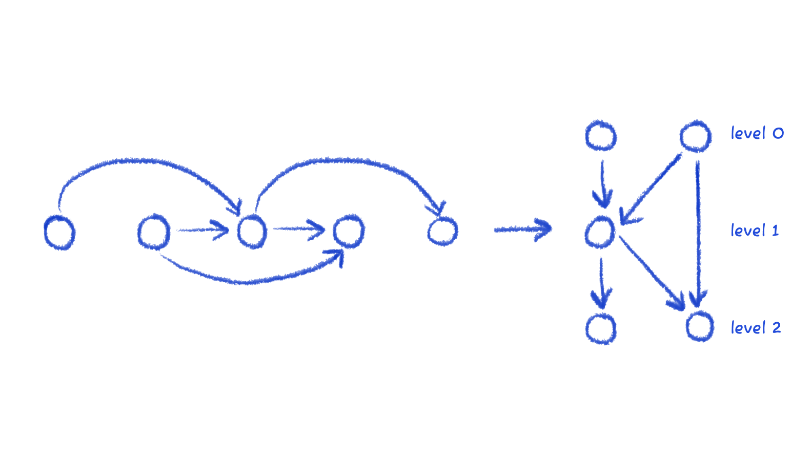
After this stage, layers are fixed, so a node cannot move up or down layers. The only thing they do in crossing minimization is move within its own layer.

A two-phase approach

TALA's method for minimizing edge crossing is separated into two phases.

Phase 1: Layer by layer crossing minimization

If we're going to run a heuristic search, we need to first define the goal to minimize, something quantifiable.

Take a look at the following difference in a crossing vs non-crossing, how might you generalize?

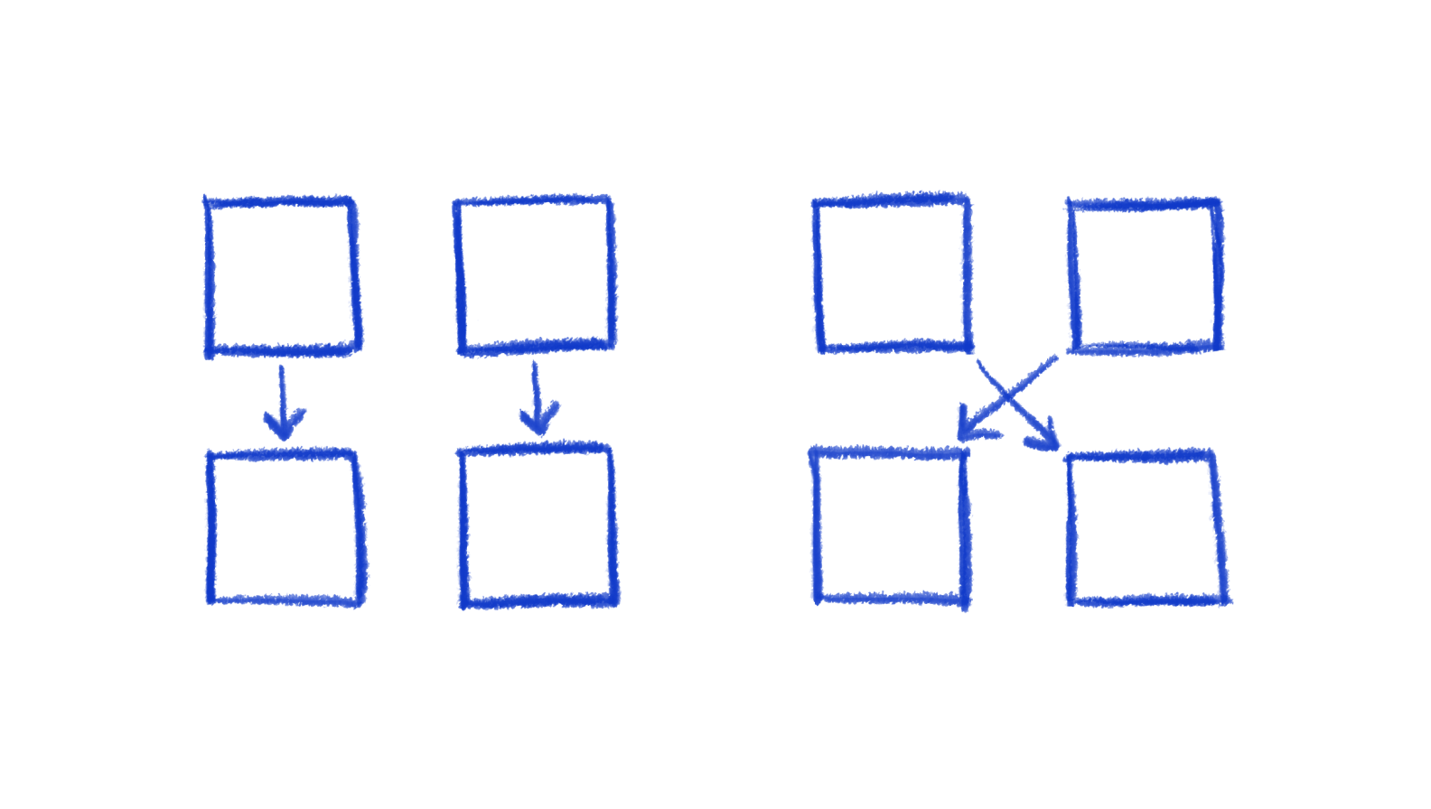
In the first diagram, the position of the node in its row (index) and its adjacent node are the same. In the second, they are swapped.

What if we add a node?

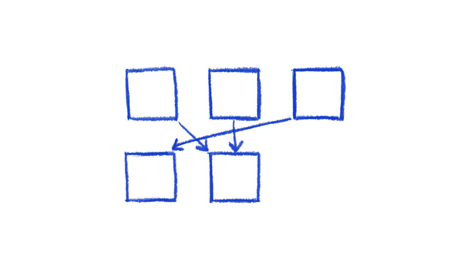
This produces one extra crossing with one of the edges, but not the other. And the edge that it created the crossing for, the index difference of the nodes increased (the top one is at index 2 while the bottom one is at index 0).

When the index difference between a node and its adjacent nodes is lower, there are fewer crossings. Let's call this difference its "adjacency delta". For example, in the above diagram, this would be the calculation for the adjacency delta of the two bottom nodes:

1. Left node: 2 (because the top node it's connected to is in position 2, and it's in position 0).
2. Right node: 0.5 (it's connected to two top nodes, at positions 0 and 1, and we just take the average, which is 0.5. The node itself is in position 1, so the delta is 0.5).

Generalized, for the entire hierarchy, we want to arrange the nodes such that the sum of the adjacency deltas for all nodes is minimized.

If we swap the bottom two nodes, the numbers change:

1. Left node: 1 (its position is 1, the top connected node position is 2, delta is 1)
2. Right node: 0.5 still

Overall, that swap decreases the sum of adjacency deltas.

What makes this a lot harder in a hierarchy is that nodes are typically interconnected. When you move one node, you're affecting multiple adjacency deltas: that node's plus all of its adjacent nodes. And it cascades.

So, instead of trying to optimize globally (consider all nodes in the hierarchy), we simplify and optimize one layer at a time in this phase.

Per layer, rearrangements happen in two more, nested, steps:

1. Consider only one side (either top or bottom) and sort based on their adjacency deltas.
2. Consider both sides, but only allow swapping with sibling neighbors to not completely overwrite step 1.

The point of having different goals is so to escape local minimas. Both of these algorithms will run layer by layer, top-down, multiple times, stopping when an optimal layout (no changes in an entire iteration) is reached or the max number of iterations is hit.

This is the pseudocode:

for i = 0 to N:
  for layer in topDown(graph):
      sortByUpperAdjacency(layer)
      for node in layer:
          bestSwap = findBestSwapNeighbor(node, layer)
          if bestSwap:
            swap(node, bestSwap)

Here's an example:

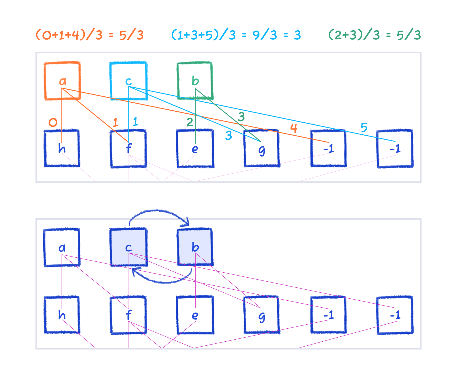
From this top layer, node a has an adjacency delta of 5/3, because its neighbors are at positions 0, 1, and 4, and the average is 5/3. Node c has 3, and node b has 5/3 as well.

So according to the algorithm, the sort will result in a, b, c.

Moving to the second layer, this is the resulting rearrangement. We won't show all the calculations again, but the sort moves one node.

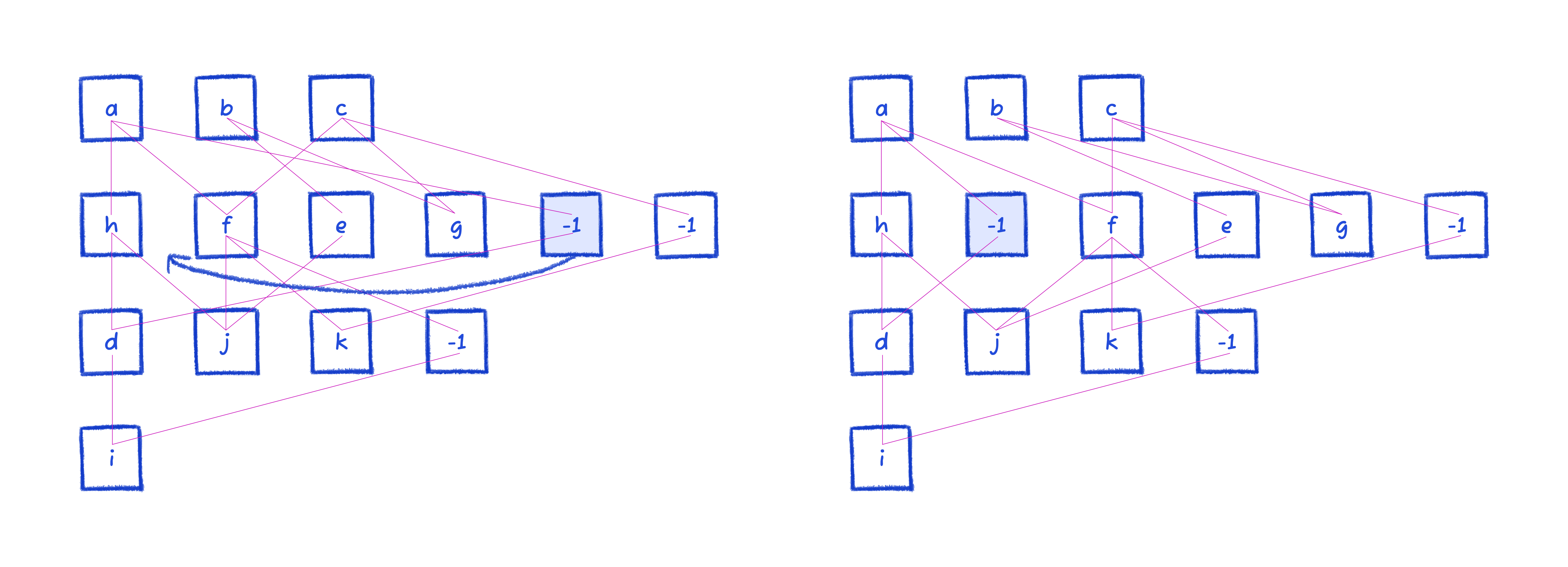
Since we're on the second layer, we look for swaps by considering both above and below.

Notice how there's a crossing between h and j, and -1 and d. Swapping h and -1 reduces their adjacency deltas, removing that crossing.

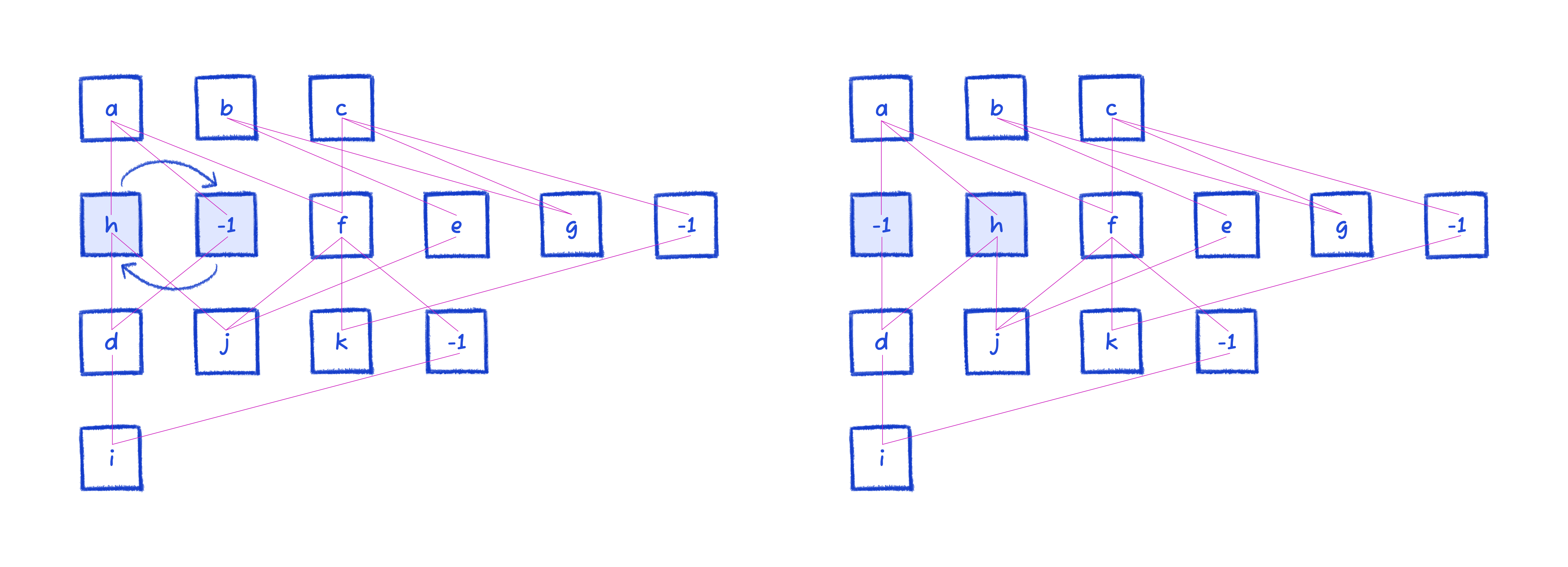
e and f can similarly be improved by swapping.

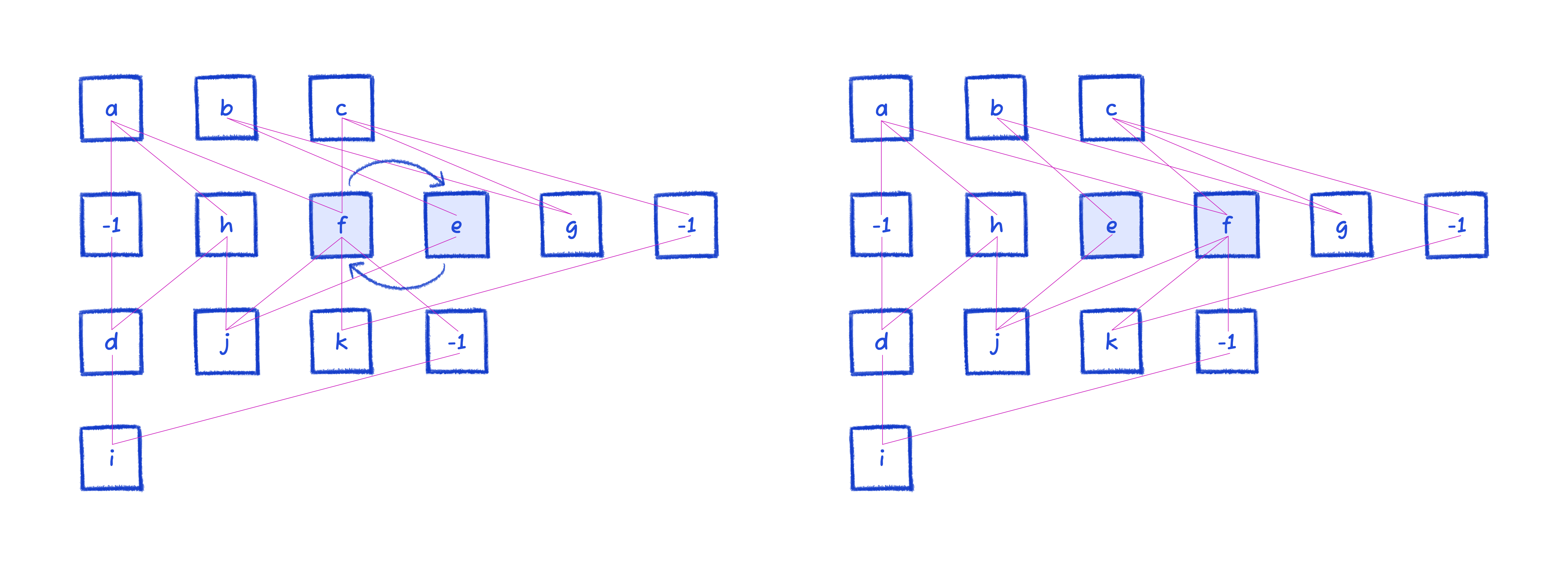
We then proceed down all the way to the bottom. Once it's made it through all the layers, that's considered one pass. We perform multiple passes (the actual number is determined by the number of layers and max width of layers).

Phase 2: Sifting

In the previous example, we converged on an optimal state after a couple passes. The layout engine still has steps to do after this, but for crossing-minimization, there is no way to rearrange for less crossings.

But that's not always the case. It could be that they just shuffle around, getting stuck at a local minima (even with the attempts to escape it).

That's what this second phase is for.

Sifting goes through the hierarchy, node by node ordered by its degree (number of connections), instead of the layer by layer approach in the first phase. For each one of these nodes, we simply check if swapping with any sibling in the same layer would result in less crossings (looking at both sides), and if so make that swap.

for i = 0 to M:
  Q = sortNodesByDegree(G)
  for node in Q:
    for sibling in layer:
       	swap(node, sibling)
        countCrossings()
        swap(sibling, node)
    moveToMinEdgeCrossings(node)

Here's an example of sifting. Note that the diagram is back to the starting position before phase 1, so that we can demonstrate on an already-familiar diagram.

The highest degree node is f, so we try swapping it among indices in its layer, keeping track of the position with the lowest crossing count.

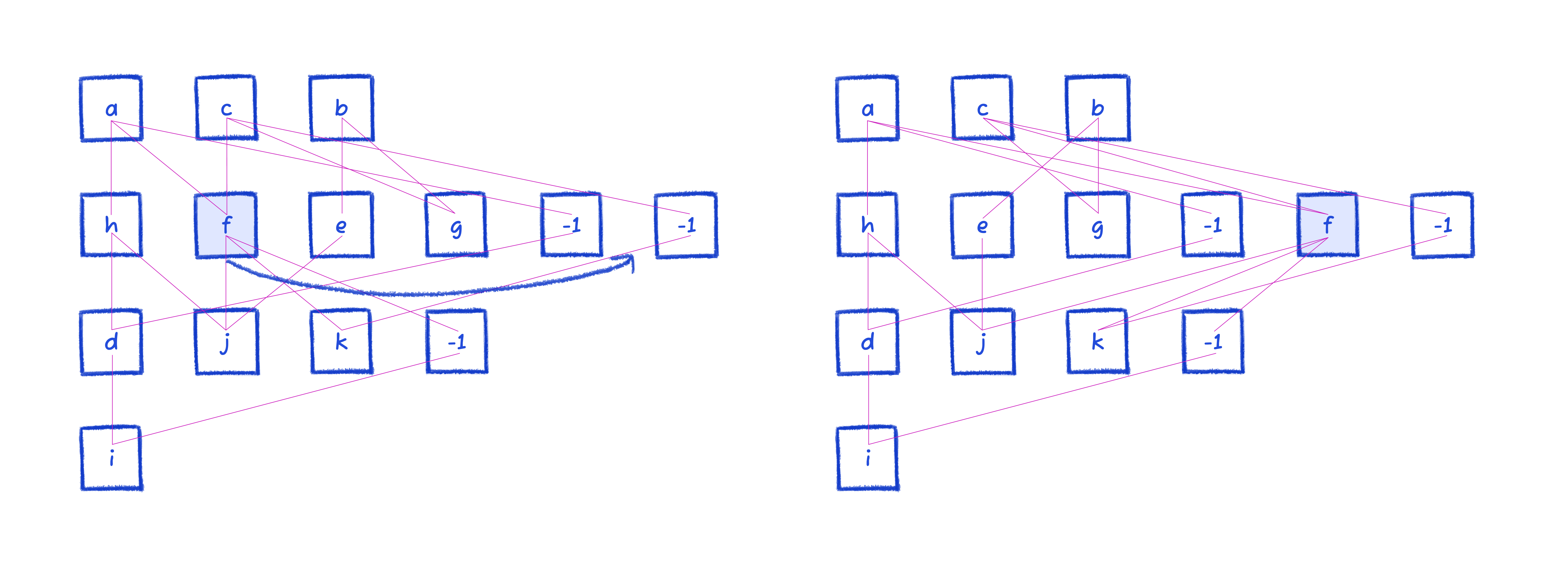
Then we move onto node a, because it has the second highest degree. It has no swaps that'd improve edge crossing count.

Next up is node c, which is swapped with b.

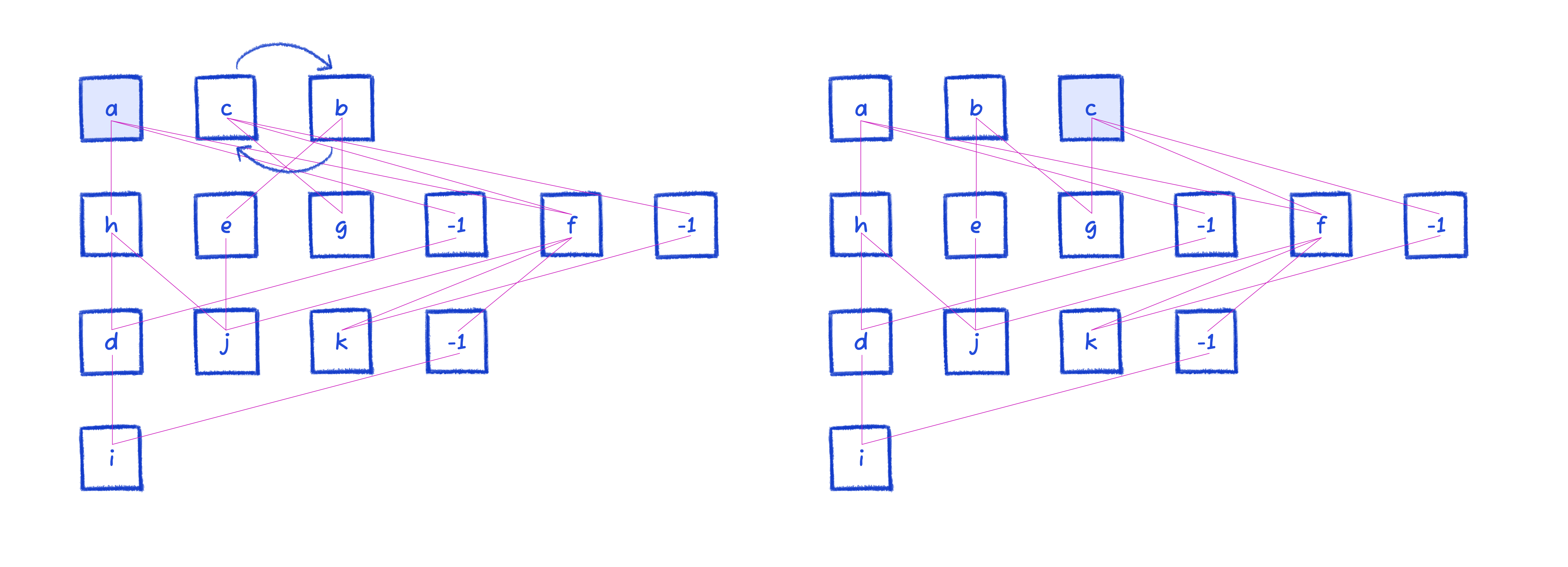
And it continues swapping nodes around until all nodes are processed. Then it repeats, so long as there were changes in the previous iterations or we reach the maximum 10 iterations.

Considering containers

TALA tests on hundreds of real-world software architecture diagrams, and we often make adjustments and considerations for that particular use case. The most common one that we constantly have to incorporate into our implementation is the support of containers. It's rarely mentioned in graph visualization publications, but it's essential for software architecture and nontrivially affects algorithms.

Here's an example of containers appearing inside hierarchies. It adds the constraint that nodes inside the container cannot move out of it, and vice versa. So, making a swap demonstrated here would be illegal.

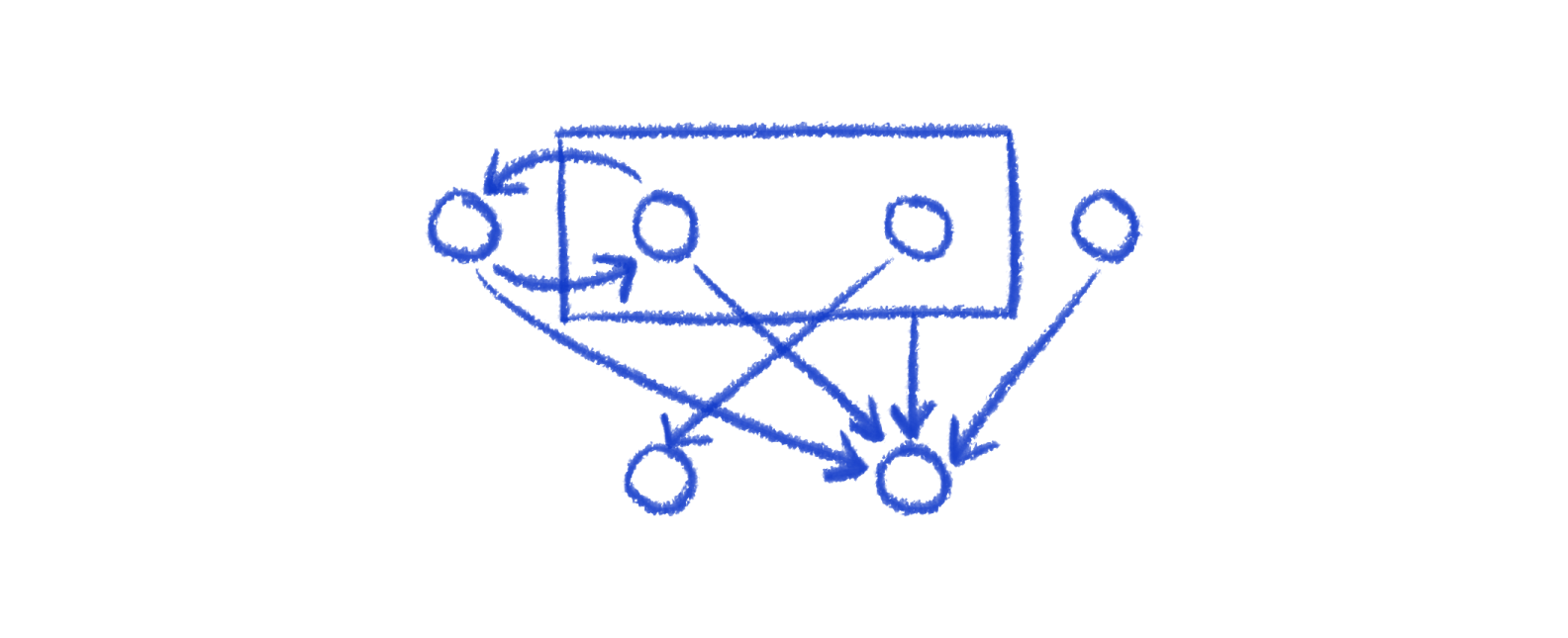
Instead of making a swap between those two nodes, we've changed the algorithm to perform grouped swaps. Instead of a single node swapping, if it's within a container, the whole container swaps with the node, carrying its descendents with it.

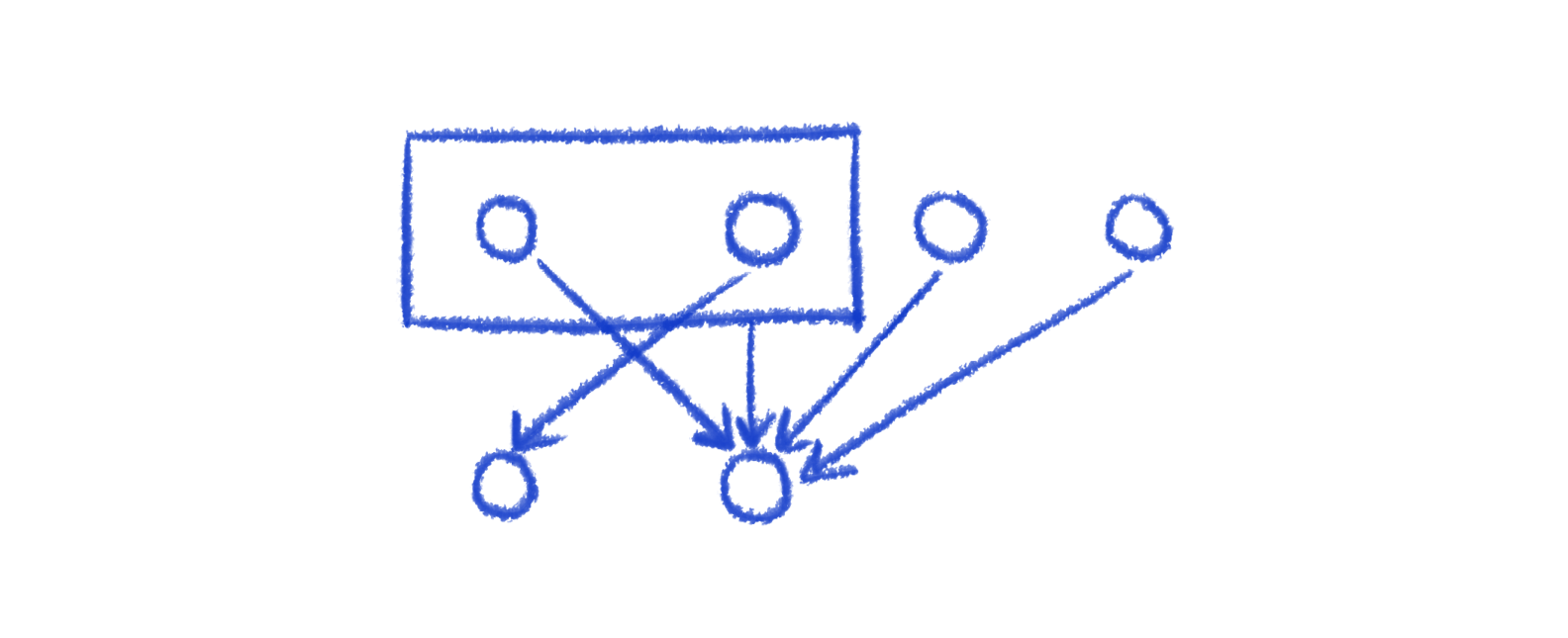
Container descendents can only order and swap among themselves.

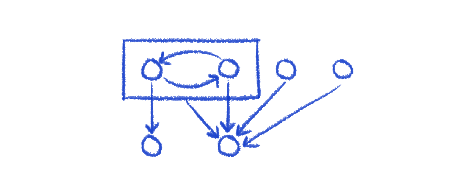
This was a straightforward change to Phase 2's sifting: just filter the list of siblings that swaps consider. However, for Phase 1, the algorithm has to change to be recursive, going from least nested to most nested nodes.

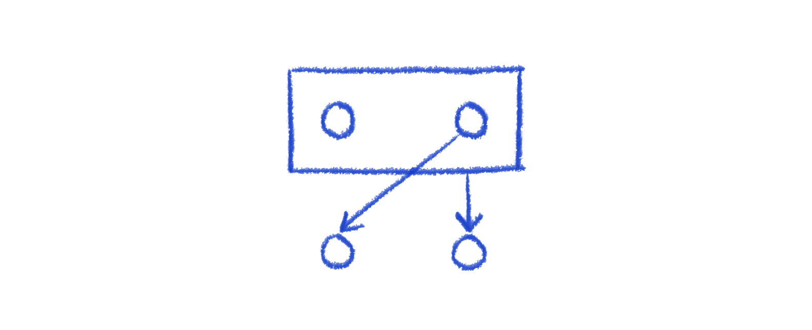
The existence of containers also opens up the possibility of a swap that doesn't decrease crossing minimizations but does decrease edge length. Consider the following. The two nodes in the container can swap for a layout with shorter edge lengths. This wouldn't be possible without containers, as the isolated node just wouldn't be part of the hierarchy.

Conclusion

There's lots of different algorithms that exist and work for hierarchical layouts. It's a cool aspect of NP-hard problems: there's generally more diversity of interesting ideas. What's more, each algorithm can have various weights and tuning, and randomization methods that further split up the breadth of results. There is no one right way. D2 bundles Dagre and ELK, which are both hierarchical layouts, and it's common for all three to give different layouts for the same diagram!

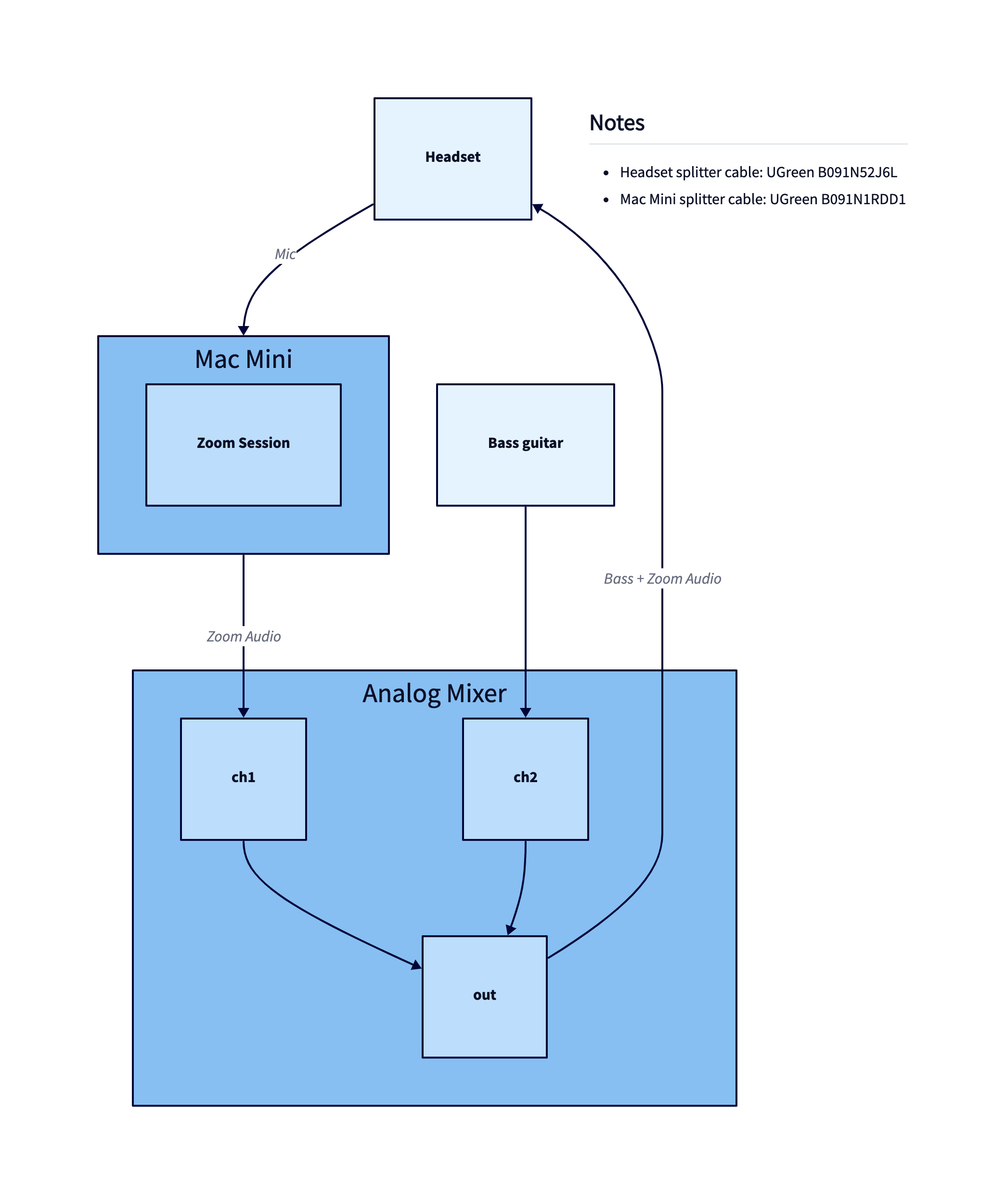
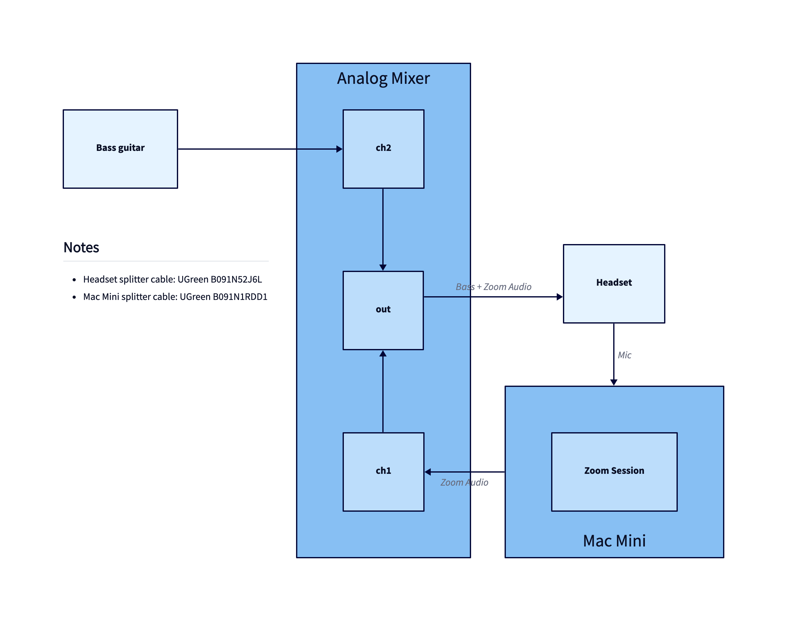
TALA's handling of hierarchies is an area of active improvement. One of those improvements is in how we identify hierarchies. There's many interesting heuristics to use, and it's a unique advantage of TALA that it can choose whether to go into the hierarchical algorithms or not. For example, in this diagram, the author did not picture a hierarchical model in their head, but using Dagre will result in a hierarchical layout regardless:

Whereas TALA chose to use an orthogonal layout instead:

If you'd like to make these diagrams yourself, it's fast and easy with D2, an open-source, modern scripting language for turning text to diagrams.

References

If you'd like to learn more:

• A Technique for Drawing Directed Graphs
• Using Sifting for k-Layer Straightline Crossing Minimization
• Handbook of Graph Drawing, Chapter 13: Hierarchical Drawing Algorithms